Accessing USGS data

This notebook does the following:

• Load a single USGS point

• Look at the metadata

• Get multiple radiation datasets

• Calculate albedo from the datasets

• Plot the albedo evolution

# imports
from datetime import datetime
import pandas as pd
import numpy as np

from metloom.pointdata import USGSPointData

# For rendering in readthedocs
import plotly.offline as py
py.init_notebook_mode(connected=True)

# Define a point known to have solar measurements
pt = USGSPointData("395709105582701", "Blue Ridge Meteorological Station NR Fraser")

# start data and end date
start_date = datetime(2024, 1, 1)
end_date = datetime(2024, 7, 1)
# Define a list of variables we want
incoming_sw = pt.ALLOWED_VARIABLES.DOWNSHORTWAVE
outgoing_sw = pt.ALLOWED_VARIABLES.UPSHORTWAVE
depth = pt.ALLOWED_VARIABLES.SNOWDEPTH
variables = [incoming_sw, outgoing_sw, depth]

# LETS GET THAT DATA
df = pt.get_hourly_data(start_date, end_date, variables)
df.head(10)

/home/docs/checkouts/readthedocs.org/user_builds/metloom/envs/stable/lib/python3.10/site-packages/metloom/pointdata/usgs.py:216: FutureWarning:

In a future version of pandas, parsing datetimes with mixed time zones will raise an error unless `utc=True`. Please specify `utc=True` to opt in to the new behaviour and silence this warning. To create a `Series` with mixed offsets and `object` dtype, please use `apply` and `datetime.datetime.strptime`

/home/docs/checkouts/readthedocs.org/user_builds/metloom/envs/stable/lib/python3.10/site-packages/metloom/pointdata/usgs.py:216: FutureWarning:

In a future version of pandas, parsing datetimes with mixed time zones will raise an error unless `utc=True`. Please specify `utc=True` to opt in to the new behaviour and silence this warning. To create a `Series` with mixed offsets and `object` dtype, please use `apply` and `datetime.datetime.strptime`

/home/docs/checkouts/readthedocs.org/user_builds/metloom/envs/stable/lib/python3.10/site-packages/metloom/pointdata/usgs.py:216: FutureWarning:

In a future version of pandas, parsing datetimes with mixed time zones will raise an error unless `utc=True`. Please specify `utc=True` to opt in to the new behaviour and silence this warning. To create a `Series` with mixed offsets and `object` dtype, please use `apply` and `datetime.datetime.strptime`

		geometry	DOWNWARD SHORTWAVE RADIATION	DOWNWARD SHORTWAVE RADIATION_units	UPWARD SHORTWAVE RADIATION	UPWARD SHORTWAVE RADIATION_units	SNOWDEPTH	SNOWDEPTH_units	datasource
datetime	site
2024-01-01 07:00:00+00:00	395709105582701	POINT Z (-105.97408 39.95258 10657)	-5.64	W/m2	-0.021	W/m2	0.616	m	USGS
2024-01-01 08:00:00+00:00	395709105582701	POINT Z (-105.97408 39.95258 10657)	-9.91	W/m2	-0.040	W/m2	0.620	m	USGS
2024-01-01 09:00:00+00:00	395709105582701	POINT Z (-105.97408 39.95258 10657)	-10.80	W/m2	-0.039	W/m2	0.618	m	USGS
2024-01-01 10:00:00+00:00	395709105582701	POINT Z (-105.97408 39.95258 10657)	-10.30	W/m2	-0.041	W/m2	0.619	m	USGS
2024-01-01 11:00:00+00:00	395709105582701	POINT Z (-105.97408 39.95258 10657)	-9.89	W/m2	-0.041	W/m2	0.620	m	USGS
2024-01-01 12:00:00+00:00	395709105582701	POINT Z (-105.97408 39.95258 10657)	-10.00	W/m2	-0.041	W/m2	0.618	m	USGS
2024-01-01 13:00:00+00:00	395709105582701	POINT Z (-105.97408 39.95258 10657)	-9.92	W/m2	-0.042	W/m2	0.619	m	USGS
2024-01-01 14:00:00+00:00	395709105582701	POINT Z (-105.97408 39.95258 10657)	-9.87	W/m2	-0.041	W/m2	0.618	m	USGS
2024-01-01 15:00:00+00:00	395709105582701	POINT Z (-105.97408 39.95258 10657)	-1.92	W/m2	3.020	W/m2	0.616	m	USGS
2024-01-01 16:00:00+00:00	395709105582701	POINT Z (-105.97408 39.95258 10657)	122.00	W/m2	55.000	W/m2	0.614	m	USGS

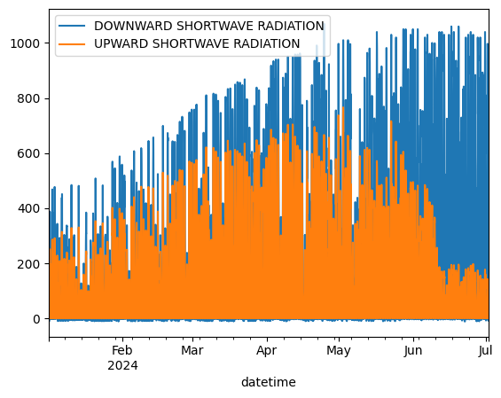
# Check out this data!
df = df.reset_index().set_index("datetime")
var_names = [v.name for v in variables]

# Sample to just the vars
df_rad = df.loc[:, var_names]

df_rad.loc[:, [incoming_sw.name, outgoing_sw.name]].plot()

<Axes: xlabel='datetime'>

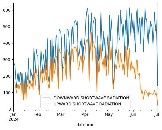
# Let's get the data in a more usable state
sw_thresh = 10

# mask the SW to decent values
df_rad[incoming_sw.name] = df_rad[incoming_sw.name].mask(df_rad[incoming_sw.name] < sw_thresh, np.nan)
df_rad[outgoing_sw.name] = df_rad[outgoing_sw.name].mask(df_rad[outgoing_sw.name] < sw_thresh, np.nan)

# Resample to daily, based on mean values
df_rad = df_rad.resample("D").mean()

# Plot again
df_rad.loc[:, [incoming_sw.name, outgoing_sw.name]].plot()

<Axes: xlabel='datetime'>

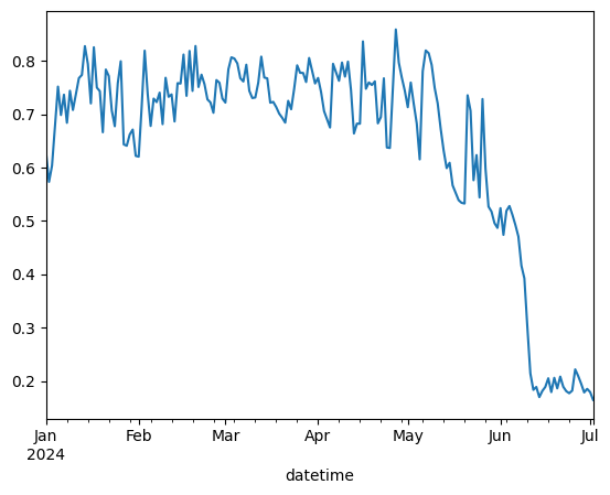
Now we can think Albedo

The daily data plot looks much better. Now we can start to think about albedo. We can use the SW to calcaulate albedo next

# Calculate albedo
albedo_var = "ALBEDO"
df_rad[albedo_var] = df_rad[outgoing_sw.name] / df_rad[incoming_sw.name]
df_rad[albedo_var] = df_rad[albedo_var].mask(df_rad[albedo_var] < 0.1, np.nan)
df_rad[albedo_var] = df_rad[albedo_var].mask(df_rad[albedo_var] > 1, np.nan)
df_rad[albedo_var].plot()

<Axes: xlabel='datetime'>

Better plotting

Awesome - now we have albedo. We haven’t used snowdepth yet, so let’s create a better plot that shows how the two relate

# Get plotly for a nicer plot
# !pip install plotly
import plotly.express as px
import plotly.graph_objects as go
from plotly.subplots import make_subplots

# Create figure with secondary y-axis
fig = make_subplots(specs=[[{"secondary_y": True}]])

# Add traces
fig.add_trace(
    go.Scatter(x=df_rad.index, y=df_rad[albedo_var], name=albedo_var),
    secondary_y=False,
)

fig.add_trace(
    go.Scatter(
        x=df_rad.index, y=df_rad[depth.name].diff(), name=f"{depth.name} signal", mode="lines+markers"
    ), secondary_y=True,
)

fig.add_trace(
    go.Scatter(
        x=df_rad.index, y=df_rad[depth.name], name=f"{depth.name}", opacity=0.3,
    ), secondary_y=True,
)

fig.update_layout(
    # template='plotly_dark',
    title=f'{pt.name}',
    xaxis=dict(title='Date'),
    yaxis=dict(
        title=f'Unitless',
        titlefont=dict(color='blue'),
        tickfont=dict(color='blue'),
        tickvals=[.25, .5, .75, 1.0],
        range=[.25, 1]
    ),
    yaxis2=dict(
        title=f'[m]',
        titlefont=dict(color='red'),
        tickfont=dict(color='red'), overlaying='y', side='right'
    )
)

# Show the plot
fig.show()

Summary

• We started with a point that we knew had shortwave measurements.

• Next, we pulled all the necessary data, cleaned it, and resampled to daily.

• We calculated albedo, and plotted it to see how the snow